Interpreting results
Use this page after a test has reached Completed and you have opened the results panel. It explains each figure on the KPI row, the confidence interval, the charts, and the data-freshness caveats that determine when a reading is trustworthy.
Before you start
- The test has completed, and the results panel has been opened at least once
- At least 2 to 3 days have passed since the test end date, so MMP attribution has caught up
- Viewer role or higher
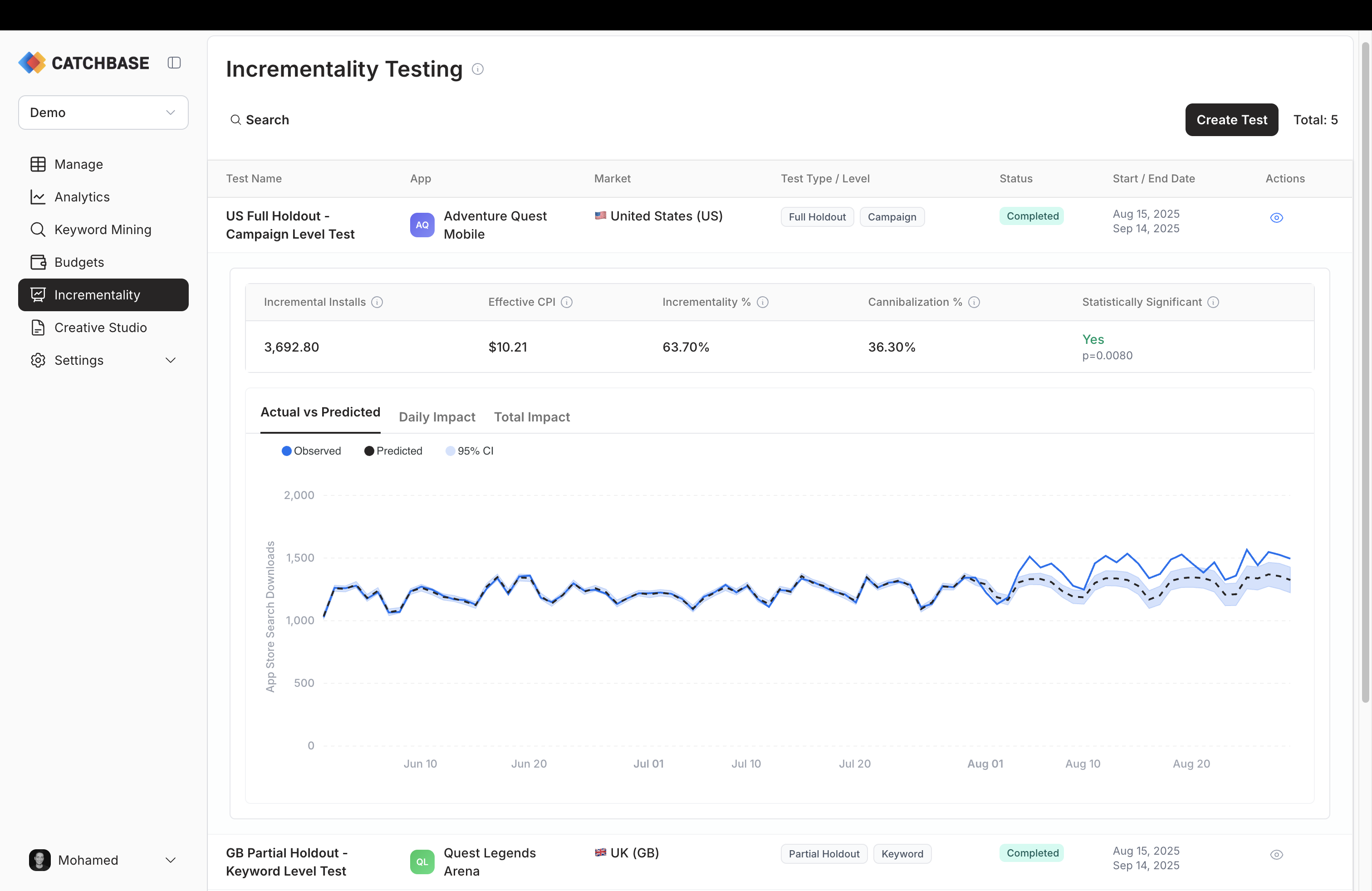
Headline figures
The results panel shows five KPIs across the top of the expanded row.
- Incremental Installs. The estimated absolute lift over the test period, in installs. This is the number of installs attributed to paid ads that the model believes would not have happened without the test-period ad activity.
- Effective CPI. Total spend during the test period divided by incremental installs. This is the true cost of an install caused by the campaign, as distinct from the blended CPI reported on the dashboard.
- Incrementality %. The share of paid installs over the test period that are estimated to be incremental.
- Cannibalization %. The complement of incrementality. The share of paid installs that would have happened anyway, through organic search or other channels.
- Statistical significance. Whether a measurable effect was detected during the intervention compared to before, shown alongside the p-value.
Relative effect and the 90% confidence interval
Below the headline figures, the analysis reports the relative effect (the lift expressed as a percentage of the counterfactual) and a 90% confidence interval for both the absolute and relative effect. The 90% interval means that, under the model's assumptions, the true effect lies inside that range in 90 percent of cases. The point estimate is a median. A wider interval means more uncertainty. Very short tests, volatile pre-test periods, or small install volumes all tend to produce wider intervals.
Charts
Three tabs show the behaviour over time.
- Actual vs Predicted plots the observed install series against the counterfactual forecast. Divergence between the two after the intervention date is the visible signal of lift.
- Daily Impact shows the daily point effect (observed minus predicted) with its own interval band.
- Total Impact shows the cumulative effect across the test period, with an interval that widens as days accumulate.
Read them together. A consistent daily impact that accumulates in the same direction is a stronger signal than a noisy daily series that happens to add up.
How the confidence interval is produced
The method is CausalImpact, a Bayesian structural time series model. To stabilise the estimate, the analysis is run multiple times on varying constructions of the control data and the reported metrics are consolidated across those runs. This produces a 90% confidence interval that reflects both model uncertainty and the sensitivity of the estimate to the choice of control data. The result shown in the panel is the consolidated reading; individual runs are not surfaced.
P-value and significance
The result reports whether a measurable effect was detected during the intervention compared to the pre-test period. When the p-value is below 0.05, the measured lift is unlikely to be due to random variation under the model's assumptions. Read it alongside the confidence interval and the daily impact chart, not on its own.
A few practical notes:
- No detected effect doesn't mean the campaign isn't working. Short tests on small budgets often don't carry enough signal to confirm an effect even when there is a real one.
- A detected effect with a wide confidence interval is weaker than one with a narrow interval. Read both.
- A small but detectable lift is not automatically worth acting on. Weigh the size of the effect against the cost of acting.
Data-freshness caveats
Two timing effects matter.
First, MMP attribution has a 1 to 2 day latency. Installs that happened in the last day or two of the test period may not have landed in the data yet. If you analyse the test on its end date, the last days will look artificially low. Wait 2 to 3 days after the test end before reading the result.
Second, revenue cohorts mature more slowly than install counts. Incrementality results here are computed on installs, not on revenue. If you want a revenue-informed reading, see Revenue and cohorts for cohort maturity windows and Data freshness for the general latency picture.
If you first opened the results before the data had matured, re-run the analysis once more post-period data has arrived. The refreshed result replaces the cached one.